Problem Description
Implementation of the Jacobi Sweep
Initialization of the Field Containing the Right-hand Side
Setting the Dirichlet Boundary Condition
Setting the Domain with an Axis-aligned Bounding Box
Outcome

Implementing an iterative solver, initializing fields, and setting Dirichlet boundary conditions by functions, domain setup with an axis-aligned bounding box. File 05_SolvingPDE.cpp.

Problem Description

After learning the basic concepts and data structures of waLBerla, we can now already implement our own solver for an elliptic partial differential equation, discretized by finite differences. The regarded equation, describing the behavior of the unknown \(u\), is:

\[ - \frac{\partial^2 u(x,y)}{\partial x^2} - \frac{\partial^2 u(x,y)}{\partial y^2} + 4 \pi^2 u(x,y) = f(x,y) \]

with the right-hand side function

\[ f(x,y) = 4\pi^2\sin(2\pi x)\sinh(2\pi y) \]

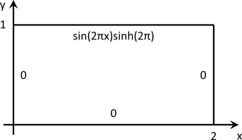
and the domain is the two-dimensional \( \Omega = [0,2] \times [0,1]\). The boundary conditions are of Dirichlet type and zero everywhere except for the top boundary, where:

\[ u(x,1) = \sin(2\pi x)\sinh(2\pi) \]

This results in the following set-up:

From basic numerical courses, we know that this equation can be discretized with finite differences which yields the following discretized equation, valid for a Cartesian grid with uniform spacing in x- \((\Delta x)\) and y-direction \((\Delta y)\):

\[ \frac{1}{(\Delta x)^2} \left(-u_{i+1,j} + 2u_{i,j} - u_{i-1,j}\right) + \frac{1}{(\Delta y)^2} \left(-u_{i,j+1} + 2u_{i,j} - u_{i,j-1}\right) + 4\pi^2 u_{i,j} = f_{i,j} \]

The resulting linear system of equations ( \(\mathbf{A}x=b\)) can be solved with either a direct or an iterative solver. Probably the simplest variant of the latter is the Jacobi method which applies a splitting of the system matrix in its diagonal and off-diagonal parts to come up with an iterative solution procedure. This finally allows to write the method in a matrix-free version, given by:

\[ u_{i,j}^{(n+1)} = \left(\frac{2}{(\Delta x)^2} + \frac{2}{(\Delta y)^2} + 4\pi^2\right)^{-1}\left[ f_{i,j} + \frac{1}{(\Delta x)^2}\left(u_{i+1,j}^{(n)} + u_{i-1,j}^{(n)}\right) + \frac{1}{(\Delta y)^2} \left(u_{i,j+1}^{(n)} + u_{i,j-1}^{(n)}\right)\right] \]

Implementation of the Jacobi Sweep

Coming back to the concepts of waLBerla, this is a perfectly suitable example for a sweep. It requires summing up weighted values of the neighboring cells together with the function value of the right-hand side, which is then divided by the weight of the center cell. To avoid data dependencies, i.e., reading neighboring data that has already been updated in a previous step, two fields (source and destination) are used like in Tutorial - Basics 3: Writing a Simple Cellular Automaton in waLBerla. After the sweep, the data pointers are swapped. A possible, but not optimal, implementation of this procedure is shown below. The class has private members srcID_, dstID_, rhsID_, dx_, dy_ that store the BlockDataIDs of the source, destination, and right-hand side field, and the grid spacings \(\Delta x\) and \( \Delta y\).

void JacobiSweep::operator()( IBlock * const block )
{
   // get the source, destination, and rhs field data from the block
   auto src = block->getData< ScalarField >( srcID_ );
   auto dst = block->getData< ScalarField >( dstID_ );
   auto rhs = block->getData< ScalarField >( rhsID_ );
 
   // iterate all cells (excluding ghost layers) of the fields
   // This macro is given a field (here src) with the matching size.
   // Inside the macro, x, y and z can be used as indices to access the data.
   // Since the three fields have the same size, these indices are valid for all of them.
   WALBERLA_FOR_ALL_CELLS_XYZ(src,
      // carries out the sweep for the current cell (x,y,z) with the respective prefactors
      dst->get(x,y,z) =  rhs->get(x,y,z);
      dst->get(x,y,z) += ( real_c(1) / (dx_ * dx_) ) * src->get( x+1,  y , z );
      dst->get(x,y,z) += ( real_c(1) / (dx_ * dx_) ) * src->get( x-1,  y , z );
      dst->get(x,y,z) += ( real_c(1) / (dy_ * dy_) ) * src->get(  x , y+1, z );
      dst->get(x,y,z) += ( real_c(1) / (dy_ * dy_) ) * src->get(  x , y-1, z );
      dst->get(x,y,z) /= ( real_c(2) / (dx_ * dx_) + real_c(2)/(dy_ * dy_) + real_c(4) * math::pi * math::pi );
   )
 
   // swap source and destination fields
   src->swapDataPointers( dst );
}

This is already the entire implementation of the Jacobi method! As always, there are of course various other ways to achieve this. The stencil concept utilized by waLBerla allows a very convenient (since flexible) and also faster implementation with the help of neighborhood iterators and stencil weights. The performance problem of the above implementation lies in the fact that the prefactors are recomputed for each step and each cell. Since they are constant, it is a better idea to precalculate them and store them in a weights vector.

typedef stencil::D2Q5 Stencil_T;
 
// set up the stencil weights
std::vector< real_t > weights( Stencil_T::Size );
weights[ Stencil_T::idx[ stencil::C ] ] = real_c(2) / ( dx * dx ) + real_c(2) / ( dy * dy ) + real_c(4) * math::pi * math::pi;
weights[ Stencil_T::idx[ stencil::E ] ] = real_c(-1) / ( dx * dx );
weights[ Stencil_T::idx[ stencil::W ] ] = real_c(-1) / ( dx * dx );
weights[ Stencil_T::idx[ stencil::N ] ] = real_c(-1) / ( dy * dy );
weights[ Stencil_T::idx[ stencil::S ] ] = real_c(-1) / ( dy * dy );

A new class JacobiSweepStencil is implemented that takes this weights vector and stores it as its private member weights_. The actual sweep, again implemented as a functor, can then be written as:

void JacobiSweepStencil::operator()( IBlock * block )
{
   // get the source, destination and rhs field data from the block
   auto src = block->getData< ScalarField >( srcID_ );
   auto dst = block->getData< ScalarField >( dstID_ );
   auto rhs = block->getData< ScalarField >( rhsID_ );
 
   // iterate all cells (excluding ghost layers) of the fields and carry out the Jacobi sweep
   WALBERLA_FOR_ALL_CELLS_XYZ(src,
 
      dst->get(x,y,z) =  rhs->get(x,y,z);
 
      // iterate the neighboring cells and multiply their value with the respective weight
      for( auto dir = Stencil_T::beginNoCenter(); dir != Stencil_T::end(); ++dir )
         dst->get(x,y,z) -= weights_[ dir.toIdx() ] * src->getNeighbor(x,y,z,*dir);
 
      dst->get(x,y,z) /= weights_[ Stencil_T::idx[ stencil::C ] ];
   )
 
   // swap source and destination fields
   src->swapDataPointers( dst );
}

At this point, another very common performance optimization strategy can be applied: to omit the costly division by the center weight in the last step of the Jacobi sweep, this weight is already stored in inverse form to allow a fast multiplication later on. The constructor of this class then looks like this:

JacobiSweepStencil( const BlockDataID & srcID, const BlockDataID & dstID, const BlockDataID & rhsID, const std::vector< real_t > & weights )
      : srcID_( srcID ), dstID_( dstID ), rhsID_( rhsID ), weights_( weights )
{
   // store the center weight in inverse form to avoid divisions in the sweep
   weights_[ Stencil_T::idx[ stencil::C ] ] = real_c(1) / weights_[ Stencil_T::idx[ stencil::C ] ];
}

And the respective line of code in the Jacobi sweep has to be changed accordingly:

...
// When the center weight is stored in inverse form, a multiplication instead of a division can be applied here.
dst->get(x,y,z) *= weights_[ Stencil_T::idx[ stencil::C ] ];
...

Despite being faster, the implementation using the stencil concept is more flexible than the hard coded variant from the beginning since it can be used for different stencil layouts. Say you use a different, probably higher-order, discretization of the PDE and come up with a D2Q9 stencil. Then, simply change the typedef to typedef stencil::D2Q9 Stencil_T and add the new weight values in the weights vector accordingly. The implementation of the JacobiSweepStencil class stays untouched and the simulations can readily be carried out.

This functor is now added to the time loop object as in the basic tutorials and the simulation can be started. At the moment, however, the simulation is very boring since the right-hand side is zero and so are the boundary conditions. It is easy to check that then \( u(x,y) = 0\) is the trivial solution. In the next sections, the functions to initialize those missing parts of the problem are shown.

Initialization of the Field Containing the Right-hand Side

In the first step of the sweep, the values of the rhs field are accessed. This field, of course, has to be initialized first, according to the given function f. This involves the evaluation of the physical coordinates of the cell centers to get the proper values for the x and y coordinate. Such a initialization function might look like this:

// function to initialise the field holding the right-hand side function f
void initRHS( const shared_ptr< StructuredBlockStorage > & blocks, const BlockDataID & rhsID )
{
   // iterate all blocks with an iterator 'block'
   for( auto block = blocks->begin(); block != blocks->end(); ++block )
   {
      // get the field data out of the block
      auto f = block->getData< ScalarField >( rhsID );
 
      // obtain a CellInterval object that holds information about the number of cells 
      // in x,y,z direction of the field excluding ghost layers
      CellInterval xyz = f->xyzSize();
 
      // iterate all (inner) cells in the field
      for( auto cell = xyz.begin(); cell != xyz.end(); ++cell )
      {
         // obtain the physical coordinate of the center of the current cell
         const Vector3< real_t > p = blocks->getBlockLocalCellCenter( *block, *cell );
 
         // set the right-hand side, given by the function f(x,y) = 4*PI*PI*sin(2*PI*x)*sinh(2*PI*y)
         f->get( *cell ) = real_c(4) * math::pi * math::pi * std::sin( real_c(2) * math::pi * p[0] ) *
                           std::sinh( real_c(2) * math::pi * p[1] );
      }
   }
}

With the help of the CellInterval object, an iterator that loops over the cells can be generated. The physical coordinates are then found by the getBlockLocalCellCenter function, with the block and the cell as arguments, and are stored in a three-dimensional vector p. This allows to obtain the x-coordinate with p[0] and the y-coordinate with p[1]. Thus, the function f can be evaluated at the specific cell.

Setting the Dirichlet Boundary Condition

In contrast to the basic tutorial, the domain is not periodic but has fixed Dirichlet boundaries on all sides. In waLBerla, it comes in naturally to use the ghost layers around the fields to store the Dirichlet values. Those are then accessed automatically in the sweep which loops only over the cells in the interior of the domain. This is carried out in the following function where only the values at the top boundary are set since the others are already initialized with zeros:

// function to initialize the boundaries of the source and destination fields
// The values of the Dirichlet boundary conditions are stored in the ghost layers of the outer blocks.
void initBC( const shared_ptr< StructuredBlockStorage > & blocks, const BlockDataID & srcID, const BlockDataID & dstID )
{
   // iterate all blocks with an iterator 'block'
   for( auto block = blocks->begin(); block != blocks->end(); ++block )
   {
      // The Dirichlet boundary condition is non-zero only at the top boundary.
      if( blocks->atDomainYMaxBorder( *block ) )
      {
         // get the field data out of the blocks
         auto src = block->getData< ScalarField >( srcID );
         auto dst = block->getData< ScalarField >( dstID );
 
         // obtain a CellInterval object that holds information about the number of cells 
         // in x,y,z direction of the field including ghost layers
         // Since src and dst have the same size, one object is enough.
         CellInterval xyz = src->xyzSizeWithGhostLayer();
 
         // To only loop over the top row of the cells, i.e., the ghost layer containing the domain boundary,
         // restrict the range in y-direction.
         xyz.yMin() = xyz.yMax();
 
         // iterate all cells in the top boundary with the iterator 'cell'
         for( auto cell = xyz.begin(); cell != xyz.end(); ++cell )
         {
            // obtain the physical coordinate of the center of the current cell
            const Vector3< real_t > p = blocks->getBlockLocalCellCenter( *block, *cell );
 
            // set the values of the Dirichlet boundary condition given by the function u(x,1) = sin(2*PI*x)*sinh(2*PI)
            // in the source and destination field
            src->get( *cell ) = std::sin( real_c(2) * math::pi * p[0] ) * std::sinh( real_c(2) * math::pi );
            dst->get( *cell ) = std::sin( real_c(2) * math::pi * p[0] ) * std::sinh( real_c(2) * math::pi );
         }
      }
   }
}

The principle action of setting the values is the same as shown for the right-hand side before. Notable, however, is the modification of the CellInterval object to yield an iterator that only loops over the ghost layer cells at the top boundary, obtained by yMax().

Setting the Domain with an Axis-aligned Bounding Box

As mentioned before, the values stored in the cells are regarded as being placed at the cell center. This introduces a slightly different way of setting the domain as one might be used to from node centered layouts. Our goal is to set the centers of the boundary cells, i.e. the ghost layers, directly at the Dirichlet boundaries. Since the ghost layer is an additional layer that is added around each block, the domain we have to set up is actually smaller than \(\Omega\). Convince yourself that this is correct by looking at the targeted grid layout:

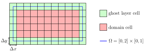
Thus, the computational domain (red) is \(\Omega_C = [\Delta x/2, 2-\Delta x/2] \times [\Delta y/2, 1-\Delta y/2]\). A convenient way to specify such a domain is the usage of an axis-aligned bounding box (aabb):

// create an axis-aligned bounding box to define domain
// defines a rectangular domain by specifying (xMin, yMin, zMin, xMax, yMax, zMax)
// care has to be taken regarding the cell-centered data layout in waLBerla
// in z-direction only one cell layer with arbitrary thickness, here dx, is present
auto aabb = math::AABB( xMin + real_c(0.5)*dx, yMin + real_c(0.5)*dy, real_c(0),
                        xMax - real_c(0.5)*dx, yMax - real_c(0.5)*dy, dx );

In waLBerla, all simulations are in principle in 3D. A two-dimensional set-up can be achieved by choosing only a single cell in z-direction with a finite cell size, here dx. The creation of the blocks is then carried out with another variant of the already known createUniformBlockGrid routine:

// create blocks
shared_ptr< StructuredBlockForest > blocks = blockforest::createUniformBlockGrid (
     aabb,                               // axis-aligned bounding box
     xBlocks, yBlocks, zBlocks,          // number of blocks in x,y,z direction
     xCells,  yCells,  zCells,           // how many cells per block (x,y,z)
     false,                              // one block per process - "false" means all blocks to one process
     false, false, false );              // no periodicity

Outcome

Putting everything together, setting up the communication scheme for the D2Q5 stencil and adding everything to the time loop, as known from the basic tutorials, the simulation can be carried out. Using the GUI, the converged profile looks like:

In the next tutorial of the PDE section, Tutorial - PDE 2: Solving the Heat Equation, the Jacobi method is used to solve the linear system of equations arising from an implicit time-stepping method for the solution of the famous heat equation. It is also shown how to include the functionality to stop the simulation based on the norm of the residual, which is very often used to terminate the iterative solver.