Tutorial - Code Generation 1: Explicit Solver for the Heat Equation

Table of Contents

• The Equation
• Building the Kernel in pystencils
• Generating a Sweep class from the kernel
• Including the generated kernel in a waLBerla application
• Outcome

This tutorial will focus on using the pystencils code generation framework for generating waLBerla sweeps. It covers the workflow for converting a partial differential equation (PDE) written as a symbolic description to a working waLBerla simulation app.

The final result of this tutorial will be a waLBerla application simulating a heat source warming up a rectangular plate from one side. In contrast to Tutorial - PDE 2: Solving the Heat Equation, we will use an explicit time-stepping scheme here.

This tutorial should not function as an introduction to pystencils itself but provide an overview of the code generation toolchain for the waLBerla framework. A detailed introduction to pystencils can be found here.

The Equation

In this tutorial, we will solve the two-dimensional heat equation which describes the flow of heat through a homogenous medium. We can write it as

\[ \frac{\partial u}{\partial t} = \kappa \cdot \Delta u \]

where \( \kappa \) is the medium's diffusion coefficient, \( \Delta \) is the Laplace operator which is short-hand for the divergence of the gradient, and \( u(x, y, t) \) is the unknown temperature distribution at the coordinate \( (x,y) \) at time \( t \). In the next section we will show how to express the equation using pystencils which builds upon sympy for describing mathematical expressions symbolically. Furthermore, we automatically derive a numerical approximation for the problem.

Building the Kernel in pystencils

For interactive devolvement, the next section can be written in a Jupyter notebook. Due to the symbolic representation provided by sympy all equations can be viewed in a \( \LaTeX \) style format.

First, we introduce the variables contained in the PDE and its discretization as symbols. For the two-grid algorithm, we require one source field u and one destination field u_tmp. Both are set as generic 2-dimensional fields. We explicitly set their memory layout to fzyx. Both waLBerla and pystencils support two kinds of memory layouts. The short fzyx lists the four domain dimensions (three spatial, one for values per cell) in the order of arrangement in memory. fzyx describes a Struct of Arrays (SOA) layout where the domain is split along f and then linearized. When iterating, the outermost loop runs over f, and the innermost loop runs over x. The alternative is an Array of Structs layout (AOS) which is designated zyxf, iterating over f in the innermost loop. In our case, where we only have one value per cell, it does not matter which layout is selected. In contrast, for simulating an Advection-Diffusion-Process with multiple, independent particle distributions, fzyx performs better in most cases as it improves data locality and enables vectorization (SIMD, SIMT). For more information on SOA and AOS, consider this article.

u, u_tmp = ps.fields("u, u_tmp: [2D]", layout='fzyx')
kappa = sp.Symbol("kappa")
dx = sp.Symbol("dx")
dt = sp.Symbol("dt")

With the pystencils buildings blocks, we can directly define the time and spatial derivative of the PDE.

heat_pde = ps.fd.transient(u) - kappa * ( ps.fd.diff( u, 0, 0 ) + ps.fd.diff( u, 1, 1 ) )

Printing heat_pde inside a Jupyter notebook shows the equation as:

\[ - \kappa \left({\partial_{0} {\partial_{0} {{u}_{(0,0)}}}} + {\partial_{1} {\partial_{1} {{u}_{(0,0)}}}}\right) + \partial_t u_{C} \]

Next, the PDE will be discretized. We use the Discretization2ndOrder class to apply finite differences discretization to the spatial components, and explicit Euler discretization for the time step.

discretize = ps.fd.Discretization2ndOrder(dx=dx, dt=dt)
heat_pde_discretized = discretize(heat_pde)

Printing heat_pde_discretized reveals

\[ {{u}_{(0,0)}} + dt \kappa \left(\frac{- 2 {{u}_{(0,0)}} + {{u}_{(1,0)}} + {{u}_{(-1,0)}}}{dx^{2}} + \frac{- 2 {{u}_{(0,0)}} + {{u}_{(0,1)}} + {{u}_{(0,-1)}}}{dx^{2}}\right). \]

This equation can be simplified by combining the two fractions on the right-hand side. Furthermore, we would like to pre-calculate the division outside the loop of the compute kernel. To achieve this, we will first apply the simplification functionality of sympy, and then replace the division by introducing a subexpression.

heat_pde_discretized = heat_pde_discretized.args[1] + heat_pde_discretized.args[0].simplify()
 
@ps.kernel
def update():
    u_tmp.center @= heat_pde_discretized
 
ac = ps.AssignmentCollection(update)
ac = ps.simp.simplifications.add_subexpressions_for_divisions(ac)

The resulting subexpression and the simplified assignment are now combined inside an AssignmentCollection. Printing ac lists the subexpression

\[ \xi_{0} \leftarrow \frac{1}{dx^{2}} \]

and the main assignment

\[ {{u_tmp}_{(0,0)}} \leftarrow {{u}_{(0,0)}} + dt \kappa \xi_{0} \left(- 4 {{u}_{(0,0)}} + {{u}_{(1,0)}} + {{u}_{(0,1)}} + {{u}_{(0,-1)}} + {{u}_{(-1,0)}}\right). \]

This completes our symbolic description of the kernel. In the next section, we will proceed to putting all of the above code inside a Python script which will then be called to generate a C++ implementation of the kernel.

Developing a numerical solver this way allows for a workflow where we can derive, test and improve our model interactively inside a Jupyter Notebook. We can use pystencils to generate and compile a parallelized kernel using OpenMP or CUDA. This kernel can then be included in small-scale prototype simulations and called as a python function. Once development on the numeric scheme itself is finished, we do not need to reimplement it in C++. Instead, we simply use the same code generation script to produce an implementation which is integrated with waLBlera for large-scale distributed-memory parallel simulations. In the tutorial folder, you can find Jupyter notebook demonstrating this workflow, including the code snippets from this section.

Generating a Sweep class from the kernel

We will now use the waLBerla build system to generate a sweep from this symbolic representation. waLBerla makes use of pystencils' code generation functionality to produce an implementation of the kernel in C. It further builds a functor class around the generated C function which can then be included into a waLBerla application.

We create a python file called HeatEquationKernel.py in our application folder. This file contains the python code we have developed above. Additionally, to sympy and pystencils, we add the import directive from pystencils_walberla import CodeGeneration, generate_sweep. At the end of the file, we add these two lines:

with CodeGeneration() as ctx:
    generate_sweep(ctx, 'HeatEquationKernel', ac)

The CodeGeneration context and the function generate_sweep are provided by waLBerla. generate_sweep takes the desired class name and the update rule. It then generates the kernel and builds a C++ class around it. We choose HeatEquationKernel as the class name. Through the CodeGeneration context, the waLBerla build system gives us access to a list of CMake variables. With ctx.gpu for example, we can ask if waLBerla was built with support for using GPUs (either by using CUDA for NVIDIA GPUs or HIP for AMD GPUs) and thus we can directly generate device code with pystencils. In the scope of this first tutorial, we will not make use of this.

The code generation script will later be called by the build system while compiling the application. The complete script looks like this:

import sympy as sp
import pystencils as ps
from pystencils_walberla import CodeGeneration, generate_sweep
 
u, u_tmp = ps.fields("u, u_tmp: [2D]", layout='fzyx')
kappa = sp.Symbol("kappa")
dx = sp.Symbol("dx")
dt = sp.Symbol("dt")
heat_pde = ps.fd.transient(u) - kappa * (ps.fd.diff(u, 0, 0) + ps.fd.diff(u, 1, 1))
 
discretize = ps.fd.Discretization2ndOrder(dx=dx, dt=dt)
heat_pde_discretized = discretize(heat_pde)
heat_pde_discretized = heat_pde_discretized.args[1] + heat_pde_discretized.args[0].simplify()
 
 
@ps.kernel
def update():
    u_tmp.center @= heat_pde_discretized
 
 
ac = ps.AssignmentCollection(update)
ac = ps.simp.simplifications.add_subexpressions_for_divisions(ac)
 
with CodeGeneration() as ctx:
    generate_sweep(ctx, 'HeatEquationKernel', ac)

As a next step, we register the script with the CMake build system. Outside of our application folder, open CMakeLists.txt and add these lines (replace codegen by the name of your folder):

if( WALBERLA_BUILD_WITH_CODEGEN )
    add_subdirectory(codegen)
endif()

The if block makes sure our application is only built if the CMake flag WALBERLA_BUILD_WITH_CODEGEN is set. In the application folder, create another CMakeLists.txt file. For registering a code generation target, the build system provides the walberla_generate_target_from_python macro. Apart from the target name, we need to pass it the name of our python script and the names of the generated C++ header and source files. Their names need to match the class name passed to generate_sweep in the script. Add the following lines to your CMakeLists.txt.

if( WALBERLA_BUILD_WITH_CODEGEN )
    walberla_generate_target_from_python( NAME CodegenHeatEquationKernel
        FILE HeatEquationKernel.py
        OUT_FILES HeatEquationKernel.cpp HeatEquationKernel.h )
endif()

The build system is now ready to generate the code. Open a terminal, navigate to the build folder of waLBerla and run the CMake configuration as shown here: Get and Build waLBerla. Make sure the flag WALBERLA_BUILD_WITH_CODEGEN is set to ON. Then, navigate to the application folder's copy inside the build directory (for this tutorial, that is build/apps/tutorials/codegen) and run make. A subfolder named default_codegen should appear, containing a C++ header and source file with the generated code. Those contain the functor class HeatEquationKernel implementing the kernel code as shown above, with the necessary boilerplate code to use it as a sweep. Just like the python kernel function, the sweep's constructor expects both fields u and u_tmp as well as the parameters dx, dt and kappa as arguments.

When running make again at a later time, the code will only be regenerated if the CMake configuration or the python script have changed. You can force CMake to re-run code generation by deleting the default_codegen folder.

Including the generated kernel in a waLBerla application

Finally, we can use the generated sweep in an actual waLBerla application. In the application folder, create the source file 01_CodegenHeatEquation.cpp. Open CMakeLists.txt and register the source file as an executable using the macro walberla_add_executable. Add all required waLBerla modules as dependencies, as well as the generated target.

walberla_add_executable (   NAME 01_CodegenHeatEquation
                            FILES 01_CodegenHeatEquation.cpp
                            DEPENDS blockforest core field stencil timeloop vtk pde CodegenHeatEquationKernel )

Open the source file and include the generated header using #include "HeatEquationKernel.h". The remainder of the application is similar to previous tutorials. We set up a two-dimensional domain by setting the physical size, number of cells and blocks for each direction. The pystencils-generated kernel expects a uniform grid with equal cell sizes in all directions. Therefore, the ratio between side length and the number of cells in each coordinate direction need to be equal. We also set the time step dt and the diffusivity coefficient kappa. Then, we create the block storage using an axis-aligned bounding box.

All of the following code snippets are added to the main function.

//  Set up the domain
//  Ensure matching aspect ratios of cells and domain.
const uint_t xCells = uint_c(25);
const uint_t yCells = uint_c(25);
 
const real_t xSize = real_c(1.0);
const real_t ySize = real_c(1.0);
 
const uint_t xBlocks = uint_c(1);
const uint_t yBlocks = uint_c(1);
 
const real_t dx = xSize / real_c( xBlocks * xCells + uint_t(1) );
const real_t dy = ySize / real_c( yBlocks * yCells + uint_t(1) );
 
WALBERLA_CHECK_FLOAT_EQUAL(dx, dy);
 
const real_t dt = real_c(1e-4);
const real_t kappa = real_c(1.0);
 
//  Axis-aligned bounding box
auto aabb = math::AABB( real_c(0.5) * dx, real_c(0.5) * dy, real_c(0.0),
                        xSize - real_c(0.5) * dx, ySize - real_c(0.5) * dy, dx );
 
//  Block storage
shared_ptr<StructuredBlockForest> blocks = blockforest::createUniformBlockGrid (
    aabb,
    xBlocks, yBlocks, uint_c(1),
    xCells, yCells, 1,
    true,
    false, false, false);

Next, we initialize both the source and destination field and create a communication scheme. Note that we explicitly set the field's memory layouts to fzyx to match the layout we specified for the kernel earlier.

//  Fields
BlockDataID uFieldId = field::addToStorage< ScalarField >(blocks, "u", real_c(0.0), field::fzyx, uint_c(1));
BlockDataID uTmpFieldId = field::addToStorage< ScalarField >(blocks, "u_tmp", real_c(0.0), field::fzyx, uint_c(1));
 
//  Communication
blockforest::communication::UniformBufferedScheme< stencil::D2Q9 > commScheme (blocks);
commScheme.addPackInfo( make_shared< field::communication::PackInfo<ScalarField> > ( uFieldId ) );

Next, let us implement the boundary conditions. We set the north domain border to a Dirichlet boundary:

\[ f(x) = 1 + \sin( 2 \pi x) \cdot x^2. \]

The northern boundary thus models an external heat source with a constant temperature distribution given by \( f \) touching our two-dimensional plate. During the simulation, this source heats the domain. We implement the Dirichlet boundary as a function which we use to initialize the domain's northernmost ghost layer to the values of \( f \). Since that ghost layer is never written to during the simulation (if we only use a single socket), we need only initialize it once. For the implementation of the Dirichlet boundary, refer to 01_CodegenHeatEquation.cpp and to Setting the Dirichlet Boundary Condition.

initDirichletBoundaryNorth(blocks, uFieldId, uTmpFieldId);

The remaining three boundaries should be Neumann boundaries imposing a normal gradient of zero, as there is no heat flow across those boundaries. We implement the Neumann boundaries using the walberla::pde::NeumannDomainBoundary class. Its constructor takes our block storage and the velocity field to which we apply the boundary condition. By default, NeumannDomainBoundary imposes the boundary condition on all six domain borders. Since a Dirichlet boundary already occupies the northern border and the simulation does not extend into the third dimension, we need to exclude the northern, bottom and top boundaries using excludeBoundary.

pde::NeumannDomainBoundary< ScalarField > neumann(*blocks, uFieldId);
 
neumann.excludeBoundary(stencil::N);
neumann.excludeBoundary(stencil::B);
neumann.excludeBoundary(stencil::T);

Last, we need to take care of swapping the source and destination fields after each iteration. We implement this as a function which we pass to the time loop inside a lambda expression.

As the last step, we set up the time loop. Passing the generated sweep to the timeloop is quite straight forward: create an instance of the HeatEquationKernel class by passing it the necessary fields and parameters, and pipe it into the timeloop. For visualizing the simulation results, we add the VTK output routine as an after-function. We set it to save one snapshot of the distribution every 200 iterations. Also, we call it once to output the initial temperature distribution.

SweepTimeloop timeloop(blocks, uint_c(2e4));
 
timeloop.add() << BeforeFunction(commScheme, "Communication") << BeforeFunction(neumann, "Neumann Boundaries")
                << Sweep(pystencils::HeatEquationKernel(uFieldId, uTmpFieldId, dt, dx, kappa), "HeatEquationKernel")
                << AfterFunction([blocks, uFieldId, uTmpFieldId]() { swapFields(*blocks, uFieldId, uTmpFieldId); },
                                "Swap");
 
auto vtkWriter = field::createVTKOutput< ScalarField, float >( uFieldId, *blocks, "temperature", uint_c(200), uint_c(0) );
vtkWriter();
timeloop.addFuncAfterTimeStep(vtkWriter, "VTK");
 
timeloop.run();
 
return EXIT_SUCCESS;

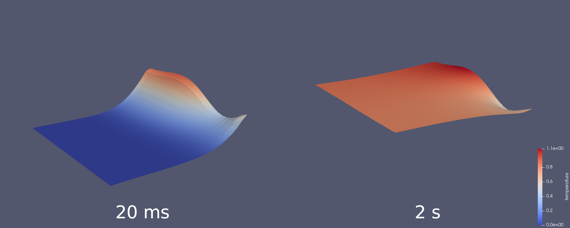
This completes our application. Below we show the temperature distribution after 20 milliseconds and after 2 seconds of simulated time.

Outcome

In this tutorial, we used the pystencils framework to discretize the heat equation and describe a numerical solver symbolically. A simulation kernel written in C was generated from the symbolic description. It was embedded in a sweep class generated by the waLBerla build system and the sweep was included in an application to simulate the flow of heat through a plate.